Step Model

Apr 27, 2020 in R
r markdown step model
4 min read

1

First divide the data into two pieces using 50:50 proportion: one for training and the other for test. (Use the last four digit of your ID as the seed number and use 50:50 proportion)

mail<-read.csv('data/directmail.csv')
mail<-na.omit(mail)
table(is.na(mail))

## 
## FALSE 
## 87543

nobs=nrow(mail)
set.seed(2059)
i=sample(1:nobs, round(nobs*0.5))
train=mail[i,]
test=mail[-i,]
nrow(train);nrow(test)

## [1] 4864

## [1] 4863

2

Fit the (1) Full Logistic Regression, (2) Stepwise Logistic Regression.

str(train)

## 'data.frame':    4864 obs. of  9 variables:
##  $ RESPOND: int  0 0 0 0 0 0 0 0 0 0 ...
##  $ AGE    : int  47 45 48 54 45 47 28 52 40 48 ...
##  $ BUY18  : int  0 1 1 0 1 0 1 0 2 0 ...
##  $ CLIMATE: int  20 30 20 20 30 20 30 10 20 30 ...
##  $ FICO   : int  692 723 677 711 694 679 682 722 710 699 ...
##  $ INCOME : int  68 19 30 28 85 68 17 54 84 49 ...
##  $ MARRIED: int  1 1 1 1 0 0 0 1 1 1 ...
##  $ OWNHOME: int  0 0 0 0 0 0 0 0 0 0 ...
##  $ GENDER : chr  "F" "M" "M" "M" ...
##  - attr(*, "na.action")= 'omit' Named int [1:273] 10 39 49 54 63 86 126 139 170 192 ...
##   ..- attr(*, "names")= chr [1:273] "10" "39" "49" "54" ...

full_model<-glm(RESPOND~AGE+BUY18+CLIMATE+FICO+INCOME+MARRIED+OWNHOME+GENDER,family='binomial',data=train)
step_model<-step(full_model, direction='both')

## Start:  AIC=2477.68
## RESPOND ~ AGE + BUY18 + CLIMATE + FICO + INCOME + MARRIED + OWNHOME + 
##     GENDER
## 
##           Df Deviance    AIC
## - INCOME   1   2459.7 2475.7
## - GENDER   1   2460.5 2476.5
## <none>         2459.7 2477.7
## - OWNHOME  1   2465.5 2481.5
## - CLIMATE  1   2469.0 2485.0
## - MARRIED  1   2470.0 2486.0
## - FICO     1   2472.0 2488.0
## - AGE      1   2482.0 2498.0
## - BUY18    1   2491.0 2507.0
## 
## Step:  AIC=2475.69
## RESPOND ~ AGE + BUY18 + CLIMATE + FICO + MARRIED + OWNHOME + 
##     GENDER
## 
##           Df Deviance    AIC
## - GENDER   1   2460.5 2474.5
## <none>         2459.7 2475.7
## + INCOME   1   2459.7 2477.7
## - OWNHOME  1   2465.5 2479.5
## - CLIMATE  1   2469.1 2483.1
## - MARRIED  1   2470.1 2484.1
## - FICO     1   2472.1 2486.1
## - AGE      1   2482.0 2496.0
## - BUY18    1   2491.0 2505.0
## 
## Step:  AIC=2474.46
## RESPOND ~ AGE + BUY18 + CLIMATE + FICO + MARRIED + OWNHOME
## 
##           Df Deviance    AIC
## <none>         2460.5 2474.5
## + GENDER   1   2459.7 2475.7
## + INCOME   1   2460.5 2476.5
## - OWNHOME  1   2466.3 2478.3
## - CLIMATE  1   2469.6 2481.6
## - MARRIED  1   2470.9 2482.9
## - FICO     1   2472.7 2484.7
## - AGE      1   2482.8 2494.8
## - BUY18    1   2491.7 2503.7

prob_pred1<-predict(full_model,newdata=test,type='response')
prob_pred2<-predict(step_model,newdata=test,type='response')
y_pred1<-as.numeric(prob_pred1>0.075)
y_pred2<-as.numeric(prob_pred2>0.075)

3

Draw a (non-cumulative) Lift Chart using R for the test data (use % Response as the Y-axis). (Do not use R packages)

#Full-model
scored1<-cbind(prob_pred1,test$RESPOND)
order_sc1<-as.data.frame(scored1[order(-prob_pred1),])
colnames(order_sc1)[2]<-'respond'
n<-round(nrow(order_sc1)/10)
lvp1=c()
for(i in 1:10){
  n1<-1+n*(i-1);n2<-n*i
  lv<-order_sc1[n1:n2,]
  lvpercent<-length(which(lv$respond==1))/nrow(lv)*100
  lvp1[i]<-lvpercent
  assign(paste0('lv1_',i),lv)
}
plot(lvp1,type='o',main='Non-Cumulative Lift Chart',xlab='Decile',ylab='Response (%)')

#Step-model
scored2<-cbind(prob_pred2,test$RESPOND)
order_sc2<-as.data.frame(scored2[order(-prob_pred2),])
colnames(order_sc2)[2]<-'respond'
n<-round(nrow(order_sc2)/10)
lvp2=c()
for(i in 1:10){
  n1<-1+n*(i-1);n2<-n*i
  lv<-order_sc2[n1:n2,]
  lvpercent<-length(which(lv$respond==1))/nrow(lv)*100
  lvp2[i]<-lvpercent
  assign(paste0('lv2_',i),lv)
}
plot(lvp2,type='o',main='Non-Cumulative Lift Chart',xlab='Decile',ylab='Response (%)')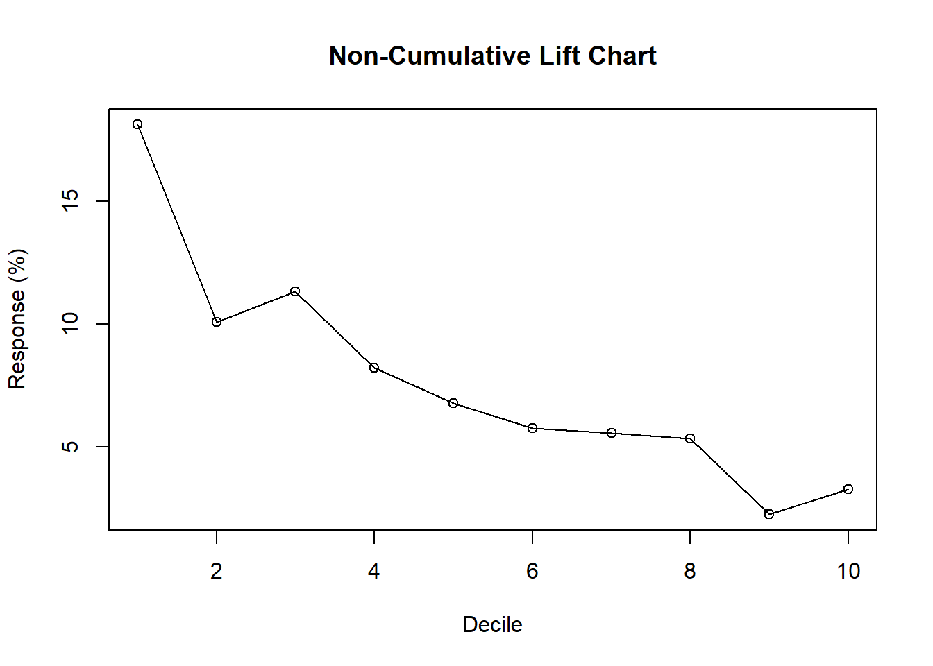

4

Draw a (cumulative) Lift Chart using R for the test data (use % Captured Response as the Y-axis). (Do not use R packages)

#Full-model
lvp1c=c()
lv1<-list()
for(i in 1:10){
  n1<-1+n*(i-1);n2<-n*i
  lv<-order_sc1[1:n2,]
  lvpercent<-length(which(lv$respond==1))/length(which(order_sc1$respond==1))
  lvp1c[i]<-lvpercent
  lv1[i]<-list(order_sc1[n1:n2,])
}
plot(lvp1c,type='o',main='Cumulative Lift Chart',xlab='Decile',ylab='Response (%)')

#Step-model
lvp2c=c()
lv2<-list()
for(i in 1:10){
  n1<-1+n*(i-1);n2<-n*i
  lv<-order_sc2[1:n2,]
  lvpercent<-length(which(lv$respond==1))/length(which(order_sc2$respond==1))
  lvp2c[i]<-lvpercent
  lv2[i]<-list(order_sc2[n1:n2,])
}
plot(lvp2c,type='o',main='Cumulative Lift Chart',xlab='Decile',ylab='% Captured Response')

5

Which model would you choose?

num=1:10
par(mfrow=c(1,2))
plot(lvp1,type='o',main='Non-Cumulative Lift Chart',xlab='Decile',ylab='Response (%)')
lines(lvp2,col=2)
abline(lm(lvp1~num))
abline(lm(lvp2~num),col=2)
legend('topright',c('Full-model','Step-model'),col=c(1,2),lwd=2)
plot(lvp1c,type='o',main='Cumulative Lift Chart',xlab='Decile',ylab='% Captured Response')
lines(lvp2c,col=2)
abline(lm(lvp1c~num))
abline(lm(lvp2c~num),col=2)
legend('bottomright',c('Full-model','Step-model'),col=c(1,2),lwd=2)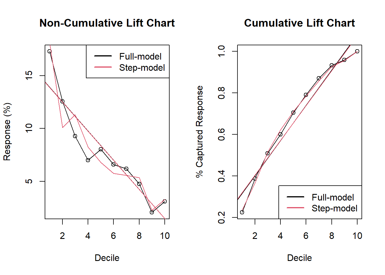

abline의 기울기가 거의 비슷하다. Decile 1~2구간에서는 Step-Model의 기울기가 더 크므로, 해당 모델을 선택하도록 한다.

6

Using the model that you chose in #5, draw a (cumulative) Profit Chart using R for the validation data under the following conditions. Fixed cost = $5,000 Cost per mailing = $7 Profit for each purchase = $100 NOTE: Calculate profits for the company (not for a person).

profit<-c()
for(i in 1:10){
  n1<-1+n*(i-1);n2<-n*i
  lv<-order_sc2[1:n2,]
  income<-length(which(lv$respond==1))*100
  cost<-5000+7*nrow(lv)
  profit[i]<-income-cost
}
plot(profit,type='o',main='Cumulative Profit Chart')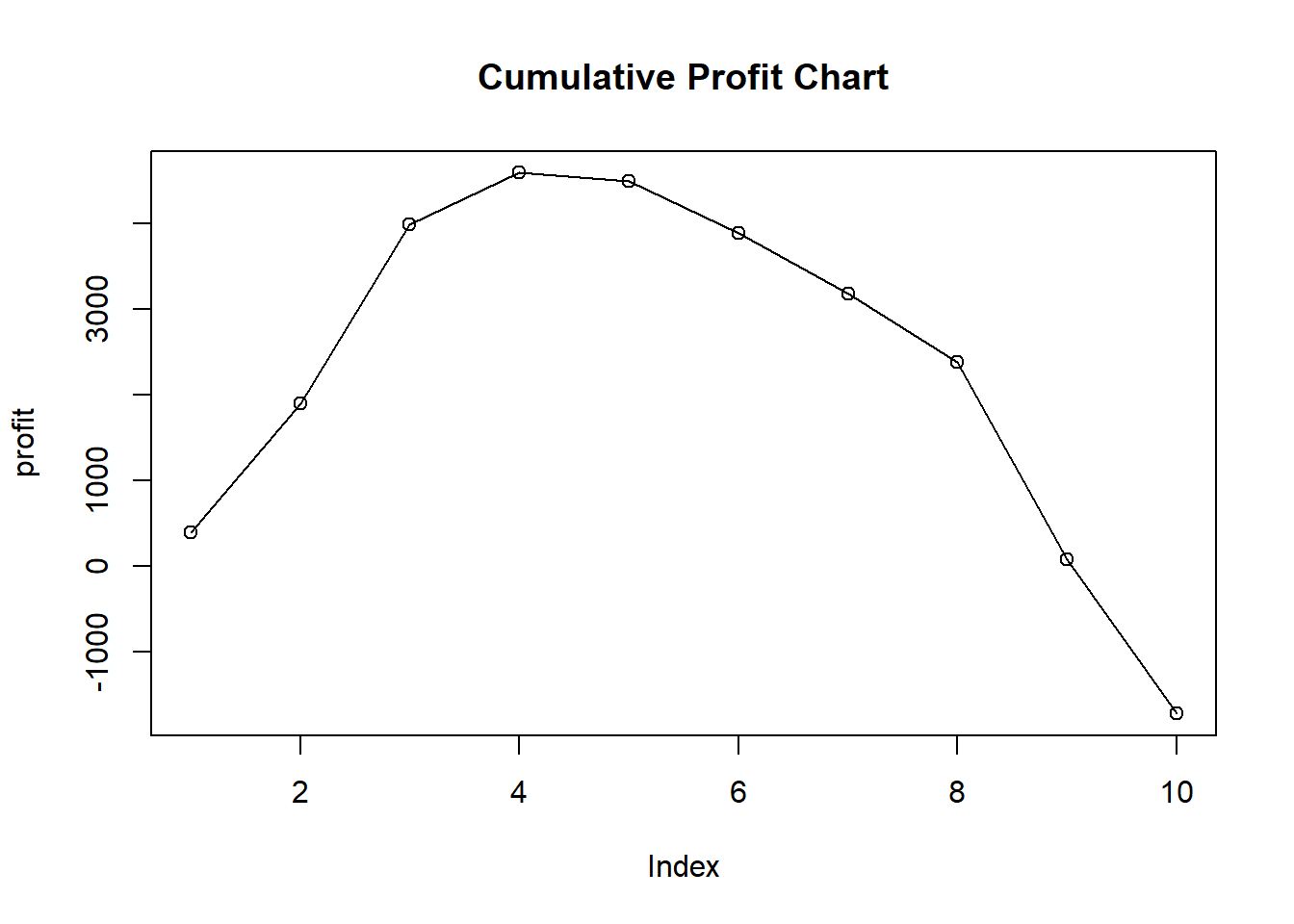

7

Suggest the proportion of ‘likely-to-buy’ customers to mail out the mailings, using the result in #6.

Decile 1 부터 증가하고 4에서 Response가 최대가 되므로 decile 4까지를 대상으로 하는 것이 적절하다.