Random Forest

Jun 30, 2020 in R
r markdown randomforest ensemble
2 min read

random forest는 Bagging을 이용한 ensemble 기법 중 하나다. 변수의 임의추출을 통해 ensemble의 다양성을 확보한다. 즉 Bootstrap Bagging과 변수 임의추출을 조합한 기법이다. tree개수가 많아 해석보다는 예측에 중점을 둔 기법이며, regression과 classification 모두 가능하다. 본 포스팅에서는 classification을 진행해보도록 한다.

data불러오기

data$y<-as.factor(data$y)
nrow(data)

## [1] 2000

table(is.na(data))

## 
## FALSE 
## 22000

table(data$y)

## 
##    0    1 
##  997 1003

총 2000개의 데이터를 사용한다. 결측치는 없으며, y변수의 개수는 위와 같다.

train data, test data분할

set.seed(99)
nobs=nrow(data)
i=sample(1:nobs,round(nobs*0.5))
train=data[i,]
test=data[-i,]
nrow(train);nrow(test)

## [1] 1000

## [1] 1000

data를 train과 test data로 각 50%의 비율로 분할한다.

모델작성

library(randomForest)
set.seed(99)
rf.model=randomForest(y~.,data=train,ntree=100,mtry=5,importance=T,na.action=na.omit)

ntree : 앙상블할 tree 개수
mtry : 임의추출할 변수개수 m
- m값이 너무 작으면, 각 tree간 상관관계가 감소
- 통상 m=√p(classification), m=p/3(regression)
importance=T : importance값 포함
na.action=na.omit : NA값 있는 경우 삭제

show(rf.model)

## 
## Call:
##  randomForest(formula = y ~ ., data = train, ntree = 100, mtry = 5,      importance = T, na.action = na.omit) 
##                Type of random forest: classification
##                      Number of trees: 100
## No. of variables tried at each split: 5
## 
##         OOB estimate of  error rate: 40.1%
## Confusion matrix:
##     0   1 class.error
## 0 302 197   0.3947896
## 1 204 297   0.4071856

Out of Bag(OOB)오차 : 40.1%
OOB error rate : Bagging의 Bootstrap 복원추출 시 뽑히지 않은 데이터로 계산한 error rate

importance(rf.model,type=1)

##     MeanDecreaseAccuracy
## x1           -1.56622393
## x2           -0.47137281
## x3            0.33615124
## x4            3.39620188
## x5            0.92841275
## x6            1.35980116
## x7           11.53376356
## x8           -0.89457424
## x9            0.08658349
## x10          -0.11013834

varImpPlot(rf.model)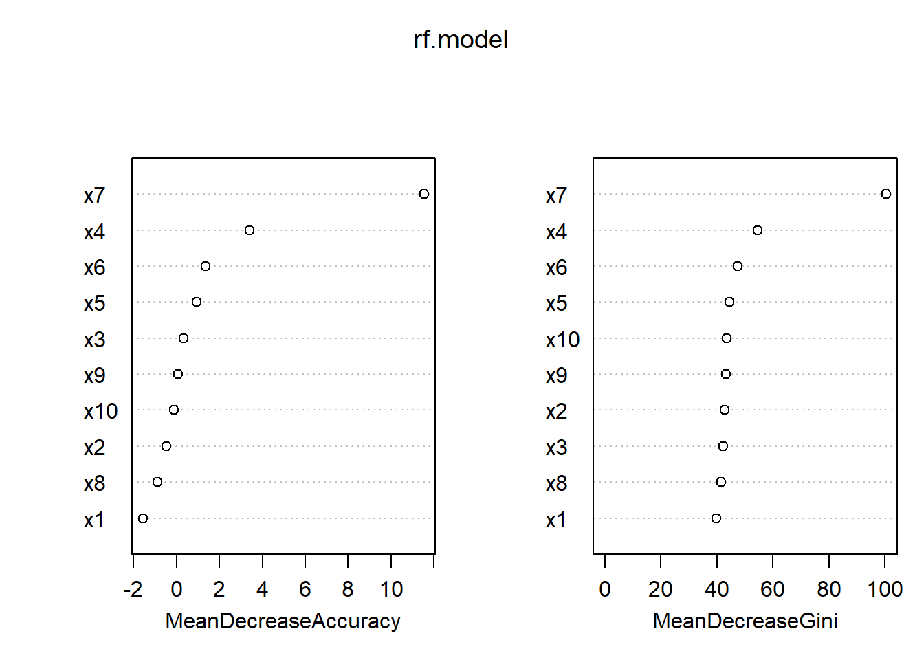

MDA(Mean Decrease Accuracy) : 관련 변수 값을 다른 값으로 대체했을 때 정확도가 감소하는 정도
X7의 MDA가 가장 높다. 즉 해당 변수가 변수들 중 가장 중요한 변수다.

모델을 이용한 예측

pred.rf.model=predict(rf.model,newdata=test)
head(pred.rf.model,10)

##  1  2  3  5 11 13 14 17 21 22 
##  1  0  1  0  1  1  0  0  0  0 
## Levels: 0 1

tab=table(test$y,pred.rf.model,dnn=c('Actual','Predicted'))
print(tab)

##       Predicted
## Actual   0   1
##      0 320 178
##      1 193 309

1-sum(diag(tab))/sum(tab)

## [1] 0.371

plot(rf.model)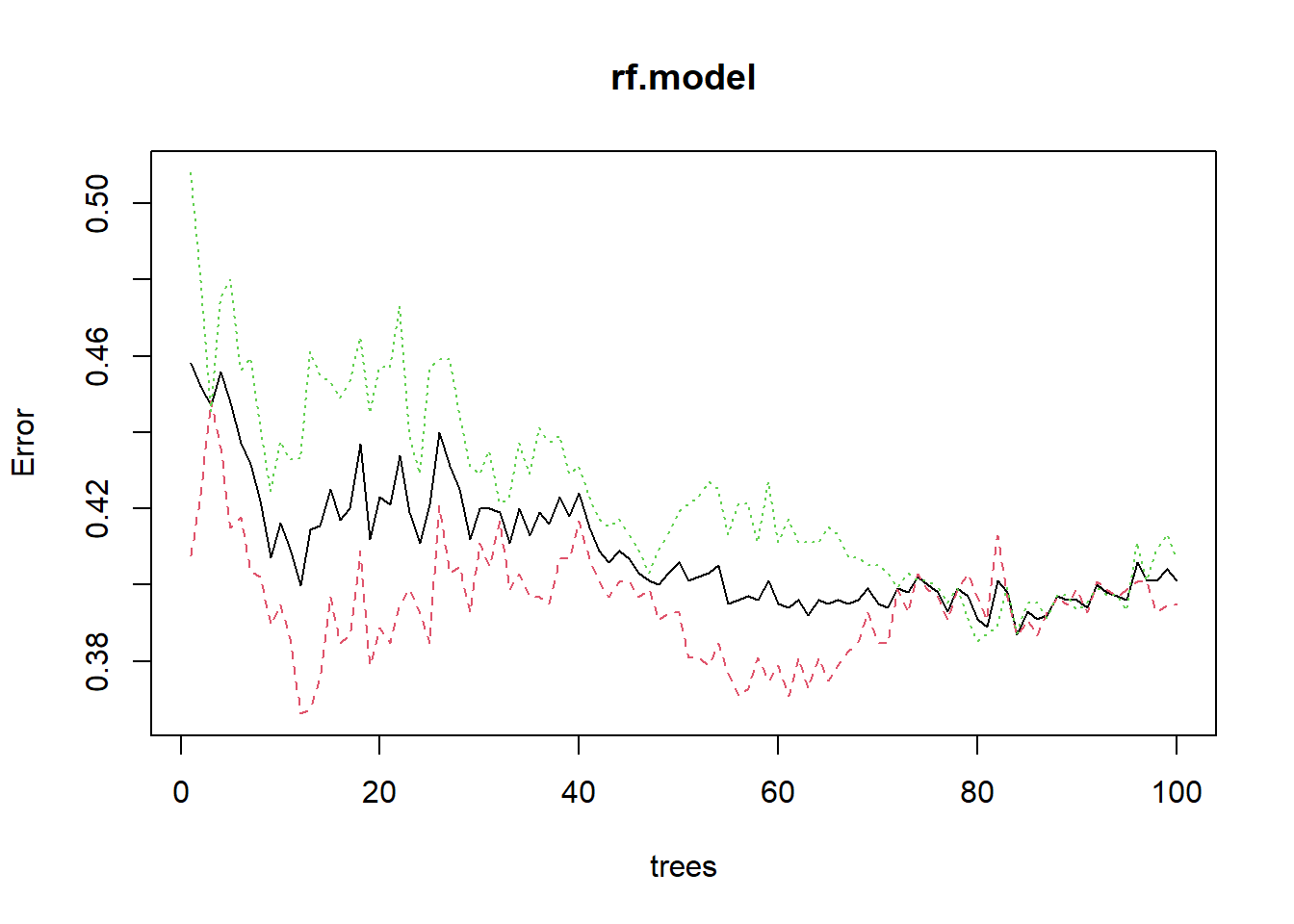

green : ‘1’ class error
black : Overall OOB error
red : ‘0’ class error

각 error는 아래와 같은 방법으로 확인이 가능하다.

head(rf.model$err.rate)

##            OOB         0         1
## [1,] 0.4582210 0.4076087 0.5080214
## [2,] 0.4519868 0.4234528 0.4814815
## [3,] 0.4469496 0.4482759 0.4456233
## [4,] 0.4559524 0.4358354 0.4754098
## [5,] 0.4478114 0.4149660 0.4800000
## [6,] 0.4371643 0.4177489 0.4562900

library(pROC)
prob.rf.model=predict(rf.model,newdata=test,type='prob')
roccurve=roc(test$y~prob.rf.model[,1])
plot(roccurve,col='red',print.auc=T,auc.polygon=T)